
Chapter 21: Query Planning and Diagnostics
Chapter 20 focused on getting data into Datalevin quickly. Once the data is loaded, performance work shifts from the write path to the read path: which query plan will run, how many facts each clause is expected to match, whether the optimizer's cardinality estimates match the current data, and what explain shows when they do not.
Datalevin's query optimizer leverages the strengths of sorted triple indexes for cardinality estimation, one of the hardest problems in database design. With that foundation, Datalevin can choose good plans for complex joins without requiring users to hand-order clauses.
A fast query depends on both the plan Datalevin chooses and the evidence you can collect when that plan surprises you. This chapter combines optimizer mechanics, recursive rule evaluation, and the explain workflow used to diagnose real query behavior.
If you are debugging a slow or surprising query right now, start with Section 3 and run explain first. Then return to Sections 1 and 2 to interpret why the planner chose a particular join order, access path, or recursive-rule strategy. Benchmark results are kept with their workload context: Chapter 1 covers JOB, Chapter 9 covers OpenRuleBench, and Chapter 13 covers LDBC SNB.
Measure the plan before rewriting the query
When a query surprises you, start with plan-only explain. It is
usually faster to inspect join order, access paths, and estimates than to guess
from clause order or rewrite a correct query blindly.
1. Query Planning and Optimization
As discussed in Chapter 8, Datalog is declarative. You describe what you want, and Datalevin's Query Optimizer decides how to find it. This decoupling is critical for performance because even a simple change in the order of joins can make a query orders of magnitude faster or slower, even though the results are the same.
This section explores how Datalevin's Cost-Based Optimizer (CBO) uses the counted indexes and ordered storage in DLMDB to create efficient execution plans.
Before a query executes its result-producing plan, Datalevin rewrites it into a simpler execution shape. Predicate pushdown, inequality conversion, constant parameter plugging, and complex-clause dependency analysis all happen before join planning. The optimizer then chooses access paths and join methods against that rewritten query.
Query optimizers evolve much like compilers and Boolean satisfiability (SAT) solvers: a stable core supports many specialized transformations and execution strategies. Datalevin follows the same pattern. New optimizations usually do not replace the storage or planning model; each recognizes another safe query shape and exposes it to the same sorted EAV and AVE indexes, counted ranges, query-specific samples, graph planner, and cost model. When a rewrite does not apply or its complete estimated cost is not lower, Datalevin retains the existing complete execution strategy. The examples below are selected to show the range and depth of Datalevin's optimizer—logical rewrites, costed access paths, physical execution, and recursive evaluation—not to inventory every optimization added in each release.
1.1 The Selinger-Style Optimizer
Datalevin uses a Selinger-style cost-based query optimizer, following the System R tradition [1]. It uses dynamic programming over join alternatives, in the same broad family as enterprise relational optimizers.
1.1.1 How it Works
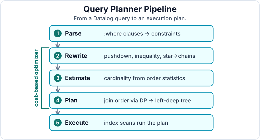
Figure 21.1 describes the query planner pipeline.
When a query is submitted:
- Parsing: The engine breaks down the
:whereclauses into individual constraints. - Rewrite and Specialization: Safe inputs become constants, indexable predicates become scan bounds, and selective bindings may be resolved before graph planning.
- Query Graph Simplification: Star-like attributes (multiple attributes on the same entity) are handled via merge scan, defined in Section 1.5, reducing the graph to chains between stars.
- Cardinality Estimation: The engine uses DLMDB's order statistics to estimate how many results each clause will produce.
- Join Planning: It explores possible join orders using dynamic programming, generating left-deep join trees.
- Bounded Search Policy: The planner keeps dynamic-programming plan tables, but shrinks the search space when the number of alternatives exceeds a cap based on the number of ordered pairs,
P(n, 2) = n * (n - 1). This keeps planning bounded while preserving careful comparison of the early joins that determine later intermediate sizes.
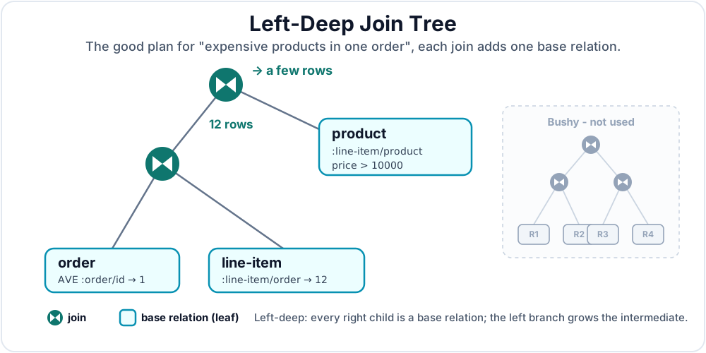
A left-deep join tree is a plan shape where each step joins one new base relation into the intermediate result built so far. The alternative is a bushy tree, where two independently built subplans are joined together. Datalevin uses left-deep plans because its join methods are index-scan oriented: keeping one side as a base relation preserves accurate counts and keeps planning cost bounded [2,3].
1.1.2 A Concrete Join-Order Example
Join order matters because every join produces an intermediate relation. A bad plan can create millions of temporary candidates and then throw almost all of them away. A good plan starts with the most selective facts and keeps the intermediate relation small.
Suppose an e-commerce database has:
- 10,000,000 orders.
- 80,000,000 line items.
- 500,000 products priced above
$100, stored as10000cents. - A unique order id, so
:order/idlookup returns exactly one order. - About 12 line items per order.
The logical query is simple: "For one order, find the expensive products in its line items."
(d/q '[:find ?sku ?qty
       :in $ ?order-id
       :where
       [?order :order/id ?order-id]
       [?line :line-item/order ?order]
       [?line :line-item/product ?product]
       [?line :line-item/quantity ?qty]
       [?product :product/sku ?sku]
       [?product :product/price ?price]
       [(> ?price 10000)]]
     db
     "o-2026-000001")
Object result = conn.query("[:find ?sku ?qty " +
    " :in $ ?order-id " +
    " :where " +
    " [?order :order/id ?order-id] " +
    " [?line :line-item/order ?order] " +
    " [?line :line-item/product ?product] " +
    " [?line :line-item/quantity ?qty] " +
    " [?product :product/sku ?sku] " +
    " [?product :product/price ?price] " +
    " [(> ?price 10000)]]",
    "o-2026-000001");
from datalevin import q

(sku, quantity, order_id, order, line, product, price) = map(
    q.var,
    ("sku", "qty", "order-id", "order", "line", "product", "price"),
)
result = conn.query(q.query(
    find=q.relation(sku, quantity),
    inputs=[q.DB, order_id],
    where=[
        q.datom(order, "order/id", order_id),
        q.datom(line, "line-item/order", order),
        q.datom(line, "line-item/product", product),
        q.datom(line, "line-item/quantity", quantity),
        q.datom(product, "product/sku", sku),
        q.datom(product, "product/price", price),
        q.predicate(">", price, 10000),
    ],
), "o-2026-000001")
import { q } from "datalevin-node";

const sku = q.var("sku");
const quantity = q.var("qty");
const orderId = q.var("order-id");
const order = q.var("order");
const line = q.var("line");
const product = q.var("product");
const price = q.var("price");
const result = await conn.query(q.query({
  find: q.relation(sku, quantity),
  inputs: [q.DB, orderId],
  where: [
    q.datom(order, "order/id", orderId),
    q.datom(line, "line-item/order", order),
    q.datom(line, "line-item/product", product),
    q.datom(line, "line-item/quantity", quantity),
    q.datom(product, "product/sku", sku),
    q.datom(product, "product/price", price),
    q.predicate(">", price, 10000)
  ]
}), "o-2026-000001");
These clauses have one logical meaning, but the physical join order can be wildly different.
| Plan step | Good plan: start from order id | Approx. candidates |
|---|---|---|
| 1 | AVE lookup [:order/id "o-2026-000001"] |
1 order |
| 2 | Reverse AVE lookup for :line-item/order |
12 line items |
| 3 | Join each line item to its product | 12 products |
| 4 | Check each product's price | a few rows |
The good plan does work proportional to one order.
| Plan step | Bad plan: start from product price | Approx. candidates |
|---|---|---|
| 1 | AVE range scan for :product/price > 10000 |
500,000 products |
| 2 | Find line items for those products | millions of line items |
| 3 | Join those line items to orders | millions of order links |
| 4 | Keep only order "o-2026-000001" |
same final rows |
The result is identical, but the bad plan may process millions of candidates to answer a question about one order. This is why Datalevin invests in cardinality estimation and join planning. The textual order of :where clauses does not matter; the optimizer is choosing this physical order for you.
The good plan is a left-deep tree: the optimizer starts from the single order, then folds in one base relation at a time, keeping the intermediate result small at every step. Figure 21.2 shows the tree for the example above.
1.2 Accurate Cardinality Estimation
The quality of a query plan depends on accurate cardinality estimates. Datalevin excels here because counting is cheap in its nested triple storage. The resulting join order is often similar to a hand-written join plan.
1.2.1 Direct Counting
Some counts can be obtained in O(1) time directly from the index without scanning. For example, [?e :user/city "London"] returns an exact count from the AVE index. For range queries, DLMDB's order statistics provide O(log n) counting.
1.2.2 Query-Specific Sampling
Direct counts are most useful for individual indexed clauses and range bounds. After several clauses have been joined, the next estimate depends on the size and distribution of an intermediate relation. Small errors can compound: if the planner underestimates users in one city, then underestimates how many of those users have active orders, the combined estimate can become much too small. For these plan-dependent estimates, Datalevin uses online reservoir sampling under actual query conditions. This is query-time work, not a background histogram. It:
- Collects sample entity ids
- Performs merge scans to get selectivity ratios
- Applies a conservative envelope to sampled fan-out estimates
The envelope is the statistical guardrail. For a sampled link, the planner uses the largest of the query-local sample mean, the storage-derived default fan-out for that attribute, and a minimum fan-out of one. This prevents a small or unrepresentative sample from producing an overly optimistic join estimate.
1.2.3 Directional Estimation
Many relational optimizers fall back to independence assumptions when they lack multi-column or join-specific statistics. Datalevin's estimation is directional because different join directions produce different estimates. This matters for :ref and :_ref joins, where starting from the source entity or the referenced value can have very different selectivity.
Planner statistics are counts and samples
Datalevin uses exact index counts, query-time sampling, per-attribute eid
samples, per-attribute cardinality counters, and default fan-out ratios. These
are not background histogram statistics, so analyze refreshes the
planner evidence Datalevin actually uses.
1.3 Query Rewrites and Predicate Push-Down
Datalevin rewrites queries to expose selective work to index scans before large intermediate relations are produced. Some rewrites become part of the query graph; others seed the graph with a small relation or reconsider work at the boundary between the main plan and late clauses.
1.3.1 Indexable Predicates and Bound Inputs
Comparison operators involving one attribute-value variable and constants are converted to AVE range boundaries. For example:
[(> ?age 21)] ;; Becomes a range scan with an open lower bound at 21
Equality becomes an exact range, while in and not-in can become exact or complementary ranges. A suitable like or not-like pattern contributes a prefix range and keeps a residual predicate when the range alone is not an exact test. Multiple bounds on the same variable are intersected, so the scan uses the narrowest interval and a contradictory interval can produce an empty result without reading attribute values.
Not every predicate is safe to encode as an index boundary. A single-variable predicate that cannot be converted exactly can still be attached to the value scan, while multi-variable predicates and dynamic-source expressions follow the normal dependency and late-clause paths.
Bound query inputs participate in the same rewrite:
[:find ?e ?age
 :in $ ?min-age
 :where
 [?e :user/age ?age]
 [(>= ?age ?min-age)]]
For a particular invocation, ?min-age is already known. Datalevin plugs that value into the query before planning, so the comparison can become a concrete lower bound on the AVE scan instead of remaining a separate predicate over a bound input.
1.3.2 Selective Anchors Before Graph Planning
Sometimes a selective fact is more useful as a small relation before the optimizer builds the query graph. If an input relation already binds one side of a pattern, Datalevin can perform the corresponding EAV or AVE probes, materialize the small result, and propagate the new bindings through other indexed patterns. This avoids representing a logically constrained lookup as a broad scan.
Multiple unique constants provide a related opportunity. In this path query, suppose both :node/id and :node/code are declared unique:
[:find ?start ?middle ?end
 :where
 [?start :node/id 1]
 [?end :node/code "three"]
 [?edge1 :edge/from ?start]
 [?edge1 :edge/to ?middle]
 [?edge2 :edge/from ?middle]
 [?edge2 :edge/to ?end]]
The two endpoint lookups can seed the same connected component, constraining the path from both ends instead of expanding from one endpoint and applying the other as a late filter. A missing unique value produces an empty relation and short-circuits the query. A single unique literal remains with the ordinary planner because it is already an ideal selective root.
Pre-materialization is not limited to unique attributes. A constant AVE lookup on a non-unique attribute can also be considered when its entity variable joins the rest of the query. The optimizer uses the exact AVE fan-out, projects the cost of propagating the resulting bindings, and compares the complete candidate with the unchanged plan. It materializes the lookup only when the whole path is estimated to be cheaper; a selective first lookup is not enough if its downstream expansion would be expensive.
1.3.3 Costed Reordering at the Late-Clause Boundary
Rules, disjunctions, and other binding dependencies sometimes keep useful work outside the main query graph. Datalevin can still compare a currently executable bound pattern with a compatible indexed producer among those late clauses. Two representative producers are an indexed union from an or-join and a bounded AVE range defined by lower and upper inequalities.
For example, suppose an earlier rule or disjunction has produced the current bindings for ?person, while ?from and ?to are bound query inputs. These clauses remain to be resolved:
[?message :message/hasCreator ?person]
[?message :message/creationDate ?date]
[(<= ?from ?date)]
[(< ?date ?to)]
The creator pattern can probe messages for the bound people. Alternatively, the engine can fuse the date pattern and its two inequalities into one AVE interval scan. A few bound people may make the creator probes cheaper; many bound people paired with a narrow date window may make the range cheaper. An indexed or-join presents the same kind of choice: Datalevin can form a small union with AVE point probes before expanding a broader bound pattern. These alternatives are costed with the values available at runtime, so the logical query need not encode either physical order.
These alternatives preserve a conservative fallback. If the clause shape is not eligible or the full switch cost is not lower, Datalevin keeps the dependency-ordered late plan. With measured explain, the selected runtime strategy is reported in :late-clause-decisions.
1.4 Cost-Based Top-k Access Paths
Datalevin's optimizer treats an ordered AVE scan and the idoc-match, fulltext, vec-neighbors, and embedding-neighbors query functions as physical alternatives for their logical clauses. It costs those alternatives with their residual joins and filters, propagates ordering and resumability as physical properties, and compares two complete physical alternatives:
| Plan alternative | How it consumes a candidate source | Effect of the final :limit |
|---|---|---|
| Conventional plan | Uses normal indexed clause and join execution to consume the complete logical source relation, including any source-local bound such as :top. |
Trims the final result and may reduce sort memory, but does not stop source work through the bounded access-path mechanism. |
| Access-path plan | Makes an eligible AVE, idoc, full-text, or vector source the physical driver, then applies residual joins and filters as candidates are consumed. | May stop source work once the requested final result is complete; otherwise it can return to the conventional plan. |
“Conventional” does not mean unindexed: both alternatives use Datalevin's indexes and join machinery. The distinction is normal complete source execution versus an incremental source plan whose work can be bounded by the final result demand. Merely having a specialized index does not force it to drive the query.
Glossary. Finite = the query has a positive :limit and a relation-shaped :find (plain tuples, no aggregates, pull, :with, :having, or result maps). Correlated = the function's arguments depend on a variable bound by an earlier clause. Resumable = the source can be consumed batch-wise and continued from an opaque position. A certified frontier additionally provides a bound proving that unseen candidates cannot improve the final window. Resumability alone does not imply that proof.
Two bounded execution modes are important:
- Adaptive top-k — the access path supplies the leading
:order-byproperty and a certified frontier. Datalevin reads batches until it has:offset + :limitdistinct final tuples and the frontier proves unseen candidates cannot change the window, consuming through the tie at the cutoff before applying secondary order terms. - Adaptive limit — the access path is complete and resumable but unordered. Datalevin reads batches until enough distinct final tuples survive the rest of the query. The selected window is intentionally unordered.
The current access methods expose these properties:
| Access method | Ordered top-k property | Unordered bounded use | Important condition |
|---|---|---|---|
| AVE | Attribute value ascending or descending | Complete AVE execution remains available conventionally | The leading order variable is the value in a simple default-source [?e :attr ?value] pattern, and an inequality supplies a scan boundary in that direction. |
idoc-match |
None | Complete, resumable adaptive limit | The match arguments are uncorrelated and the result uses the normal [e a v] relation shape. |
fulltext |
Score descending | Complete, resumable adaptive limit | Ranked order requires exactly one domain, :display :refs+scores, and score as the leading order term. |
vec-neighbors, embedding-neighbors |
Distance ascending | Complete, resumable adaptive limit | Ranked order requires exactly one domain, :display :refs+dists, and distance as the leading order term. |
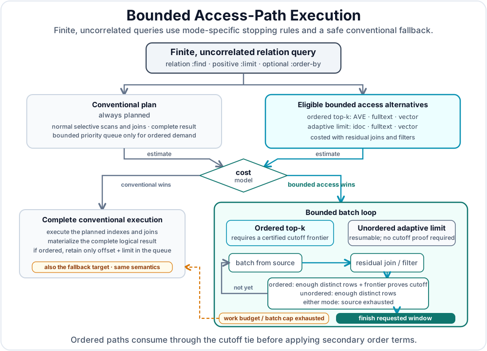
Ordered example — AVE supplies the leading order. The scan starts at the inequality boundary and proceeds backward, testing structured clauses per batch:
[:find ?title ?score
 :in $ ?max-score
 :where [?e :item/score ?score]
        [(<= ?score ?max-score)]
        [?e :item/active? true]
        [?e :item/title ?title]
 :order-by [?score :desc ?title :asc]
 :offset 20
 :limit 10]
The inequality is eligibility, not a hint about clause order. Only the leading ?score :desc comes from the AVE order; a large tie at the cutoff still requires scanning through the tie before ?title :asc is applied.
Unordered example — idoc has no ranked order but can still stop early:
[:find ?e ?name
 :where [(idoc-match $ :user/metadata {:theme "dark"}) [[?e _ _]]]
        [?e :user/name ?name]
        [?e :user/active? true]
 :limit 20]
Batches of document matches are joined and filtered until 20 distinct final tuples survive. Without :order-by the window has no ordering guarantee and an offset does not define stable pagination.
Source-local and query-level bounds remain separate. Full-text functions use :top, :limit, and :offset to bound their candidate relations; vector functions use :top. Query-level :offset and :limit apply after residual joins, filters, projection, and duplicate elimination. The optimizer can avoid consuming an unused suffix, but it never widens the source window or changes vector-search approximation and recall.
Early stopping requires a finite relation-shaped query as defined above. Correlated arguments (full-text, idoc, vector, embedding) use normal complete query-function execution. A physical join must preserve the source order for adaptive top-k; if a cheaper hash join would destroy that property, the optimizer keeps the unordered access-path plan or the conventional plan.
Adaptive execution runs under a bounded candidate budget and a hard candidate-batch safety cap, retaining the already planned conventional plan as a fallback. If either limit is exhausted before a valid stopping proof, Datalevin runs the conventional plan with unchanged semantics — for an ordered query the same window, while for an unordered limited query no stable window identity exists. Non-access-path ordered queries still use the bounded priority queue described in Chapter 8.
1.4.1 Post-Top-k Projection Enrichment
An ordered, limited query can sometimes select its result window before loading optional properties that are used only in the projection. get-some-else makes that safe because it always produces exactly one tuple: the first present [attribute value], or [nil fallback] when none of the listed attributes is present.
[:find ?id ?content ?score
 :where [?item :item/id ?id]
        [?item :item/score ?score]
        [(get-some-else $ ?item nil :item/content :item/image)
         [_ ?content]]
 :order-by [?score :desc ?id :asc]
 :limit 5]
Here :item/id is unique and remains in the projection, while ?content is not used by ordering, filtering, or another clause. The planner can therefore rank and select the five distinct rows first, then look up content only for those rows. get-some is not interchangeable in this optimization: when neither attribute is present it removes the row, which can change the selected window.
The rewrite is applied only when the planner proves that the enrichment is cardinality-preserving and projection-only, and that the retained projection contains the entity itself or a unique value identifying it. explain reports the plan and proof under :post-top-k-enrichment; measured execution also adds the candidate and selected row counts. If a proof condition is absent, Datalevin evaluates the clause in its normal position.
1.5 Merge Scan
For star-like queries (multiple attributes on the same entity), Datalevin uses merge scan, a technique similar to pivot scan [4].
Instead of joining each attribute separately, an EAV-oriented merge scan can retrieve matching attributes for the same entity in one ordered pass. The optimizer can then plan over a simplified query graph whose nodes are star-shaped groups and whose edges are links between those groups, reducing the join search space [7,8,9]. For star-heavy queries, this removes a large amount of otherwise repetitive entity-local work.
1.6 Join Methods
Datalevin considers six join methods and picks the best based on cost estimation:
| Method | Use Case |
|---|---|
Forward ref :ref |
[?e :user/friend ?f] - merge scans ref values |
Reverse ref :_ref |
[?f :user/_friend ?e] - scans AVE then retrieves entities |
Value equality :val-eq |
When variables unify via attribute values |
Hash join :hash-join |
Large non-selective joins where the cost model favors materializing a target relation |
Or-join :or-join |
Handles or-join clauses with sideways information passing (SIP) |
Not-join :not-join |
Optimizes conservative anti-join shapes instead of always deferring negative filters |
Sideways information passing (SIP) means passing already-known variable bindings from one part of the plan into another part that is not simply the next linear data pattern. In ordinary joins this happens naturally through shared variables: once ?user is bound, a later clause such as [?order :order/customer ?user] can use that value to do a narrow lookup. An or-join is more complicated because it contains several alternative branches. SIP lets the planner evaluate each branch with the outer bindings it is allowed to see, rather than evaluating every branch as an independent broad subquery and joining the results afterward.
For example, an or-join whose declared join variables include ?user can receive the current ?user bindings from earlier indexed clauses. Each branch then asks a bounded question such as "does this user match by email?" or "does this user match by phone?" instead of scanning all users that match either branch. The declared join-variable list matters: it is the contract that tells the optimizer which outer variables may be passed sideways into the alternatives and which branch-local variables must stay internal. If a complex clause cannot use the available bindings, it is less selective and may be planned later.
An anti-join is the negative counterpart of a join: it keeps a candidate row only when no matching row exists on the excluded side. In SQL this is the shape behind NOT EXISTS; in Datalevin it is usually expressed with not or not-join. A planned not-join is useful when the engine has already bound the declared join variables and can check the negative pattern with indexed lookups. For example, after ?start and ?person are bound, a not-join [?start ?person] can ask "is there a direct friendship edge between these two?" and discard the candidate only if that edge exists. The result is still declarative negation, but the physical plan can avoid treating the negative pattern as a late row-by-row filter.
In hash-join terminology, the build side is the input used to construct an in-memory hash table, and the probe side is the input scanned to look up matches in that table. Building on the smaller side usually saves memory and work. Datalevin considers a hash join when estimated intermediate sizes make repeated index probes expensive; for reverse-reference joins it can also combine hash joining with SIP when the target side is much larger than the current input.
When several links from the partial plan can reach the same next graph node, Datalevin first prefers the link from the most recently resolved source. Here, “recently” refers to its position in the partial plan, not the age of the stored data. That source is closest to the current intermediate relation, so its link estimate uses the freshest binding context; cost and estimated output size break ties among equally recent links.
1.7 Parallel Processing
Datalevin's query engine uses parallelism at several levels:
- Planning: Independent counts, samples, and connected components can be processed in parallel.
- Storage scans: Large batches for selected EAV and AVE operations can be divided among workers when their predicates are safe to run concurrently.
- Plan execution: Long eligible runs of indexed steps can use morsel-driven partition execution. Other plan segments use a bounded tuple pipeline, so downstream work can begin before the entire upstream relation is available.
1.7.1 Morsel-Driven Execution
A morsel is an independent chunk of an intermediate tuple relation. Morsel-driven means that these chunks, rather than individual plan steps, are the units scheduled across workers. For a sufficiently large input followed by a long linear run of :link and :merge steps, Datalevin divides the input into morsels and processes them concurrently [11]. Each worker carries its morsel through the remaining steps in that run. This keeps index operations batched within a partition instead of assigning a separate task to every step.
The payoff appears when an early step produces many tuples and several indexed joins remain: available cores can advance independent parts of that relation through the indexed suffix. With the current defaults, partitioning is considered at 8,000 input tuples when at least three eligible index steps remain. A target of roughly 2,000 tuples per participant bounds useful parallelism; the processor count and available common-pool capacity can reduce the participant count further. These thresholds choose an execution strategy and do not change query semantics.
The executor finds each maximal eligible run independently. A hash join, semi-join, branch, access operator, or another coordinating step ends one run, but a safe run before or after it can still be partitioned. Merge predicates must be forkable, and a merge that depends on a precomputed relation is not eligible. Writes, non-forkable predicates, small inputs, short runs, and single-core execution retain the pipelined or serial path.
Datalevin uses only one layer of parallelism inside a partitioned run. It disables storage-level chunking while a worker advances a morsel, preventing nested tasks from oversubscribing the shared pool. The caller processes one morsel while other morsels use available workers. Results are concatenated in partition order, and measured per-step row counts are summed across morsels.
Reading morsel execution in measured explain
Measured explain records each runtime split in the top-level
:partitioned-execution vector. Each entry identifies the segment
with :segment-start-step-index,
:split-step-index, and :segment-end-step-index; reports
:input-rows and :partitions; and describes the work
with :segment-step-count, :segment-step-types,
:partitioned-step-count, and
:partitioned-step-types. The optional
:previous-step-type and :next-step-type fields show
the nonlinear steps at the segment boundaries. Plan-only explain omits this
vector because the runtime split depends on the intermediate relation and
available execution capacity.
1.8 Complex Clauses and Rules
The optimizer handles complex clauses in stages:
- Index access clauses produce intermediate results first
- Heuristics and variable dependencies reorder remaining complex clauses such as
and,or,not, complex predicates, and function bindings that are not pushed down. - Rules are handled by the specialized bottom-up evaluation machinery described later in this chapter.
or-join participates in link planning, and common not-join shapes can become anti-join steps when their join variables are bound in a single plan component. More complex negative clauses still fall back to late resolution. Optimizer coverage at this boundary continues to grow: eligible indexed unions and bounded AVE ranges can now compete with an earlier bound pattern, while other clause shapes retain dependency-ordered late execution.
1.9 Optimizer Principles
In summary, Datalevin has a sophisticated query optimizer that compiles declarative query clauses into execution steps that use index scans where they help, take advantage of cheap counts from triple storage, and often produce plans similar to a hand-written one. Users can usually write the logical query first, then use explain when a specific workload needs inspection or tuning.
- Clause order does not matter for the most part: The optimizer chooses the physical order for most clauses. Deferred
:late-clausesare also re-ordered according to their binding dependencies. If two late clauses are both fully bound at the same time, their original order does matter. - Core indexes are automatic; composite access paths are explicit: Datalevin maintains EAV for every attribute and AVE unless
:db/noindexopts out. It does not invent a maintained multi-attribute value from a query shape. For a measured hot query that repeatedly consumes the same cardinality-one attributes, define a:db/tupleAttrsattribute and make the query read it explicitly. This can replace a large intermediate relation produced from component EAV datoms with the usually smaller relation of qualifying joint combinations. The cost is another indexed datom and additional work on every component update; Chapter 11, Section 1.2 compares the two IC5 query variants. - Counts are live and samples are refreshable: DLMDB gives the planner cheap current index counts, while background sampling and explicit
d/analyzecalls refresh per-attribute eid samples, per-attribute cardinality counters, and default fan-out ratios. These are not histogram-style distribution statistics. - Nested storage helps planning: The nested triple storage makes counting cheap, giving the optimizer evidence that many systems have to approximate.
- Properties are part of the choice: Ordering, resumability, completeness, frontier guarantees, and result quality determine whether an AVE, idoc, full-text, or vector alternative can satisfy the root query safely.
2. Recursive Rules as Specialized Query Evaluation
Non-recursive rules are pulled out and planned as part of the query optimization described above. Recursive rules require specialized planning because the engine may have to derive new tuples over several rounds before the rule result is complete. This section explains the separate machinery: semi-naive evaluation, deltas, and rule-specific rewrites.
(def ancestor-rules
  '[[(ancestor ?x ?y)
     [?x :person/parent ?y]]

    [(ancestor ?x ?y)
     [?x :person/parent ?z]
     (ancestor ?z ?y)]])
Object ancestorRules = Datalevin.edn("""
    [[(ancestor ?x ?y)
      [?x :person/parent ?y]]

     [(ancestor ?x ?y)
      [?x :person/parent ?z]
      (ancestor ?z ?y)]]
    """);
from datalevin import q

x = q.var("x")
y = q.var("y")
z = q.var("z")
ancestor_args = q.join_vars(x, y)
ancestor_rules = q.rules(
    q.rule_branch(
        "ancestor", ancestor_args,
        q.datom(x, "person/parent", y),
    ),
    q.rule_branch(
        "ancestor", ancestor_args,
        q.datom(x, "person/parent", z),
        q.rule("ancestor", z, y),
    ),
)
import { q } from "datalevin-node";

const x = q.var("x");
const y = q.var("y");
const z = q.var("z");
const ancestorArgs = q.joinVars(x, y);
const ancestorRules = q.rules(
  q.ruleBranch(
    "ancestor", ancestorArgs,
    q.datom(x, "person/parent", y)
  ),
  q.ruleBranch(
    "ancestor", ancestorArgs,
    q.datom(x, "person/parent", z),
    q.rule("ancestor", z, y)
  )
);
For the ancestor rule set above, a naive evaluator would repeatedly join all known ancestors against all parents. That repeats work. In the third round, for example, it may rediscover grandparent facts already found in the second round. On large graphs, this redundant computation can dominate the query.
Datalevin therefore uses semi-naive evaluation, the standard bottom-up strategy for recursive Datalog [8]. The key idea is delta tracking: each round only uses the new tuples discovered in the previous round. Evaluation continues until a fixpoint, meaning a round produces no new tuples. The engine also builds rule-dependency components and evaluates them in dependency order. A later rule component can use facts computed by an earlier component, but not the other way around. Strongly connected recursive components run to a fixpoint before dependent components consume their results.
This bottom-up model is set-oriented. Joins operate over candidate sets and iterators, so the storage layer can use sequential page scans, merge-style operations, and bulk filtering rather than tuple-at-a-time random lookup.
Bottom-up evaluation has one obvious risk: it can compute more of the world than the user asked for. If a query asks only for Alice's ancestors, the engine should not materialize every ancestor relation in the database. Datalevin uses magic-set rewriting, a classic Datalog transformation for making bottom-up evaluation goal-directed [8,9]. Magic-set rules push bound variables from the outer query into the recursive rule, pruning intermediate results to the part of the graph relevant to the question.
2.1 Semi-Naive Evaluation
Consider a small directed graph, using letters as stand-ins for entity ids. The example EDB is the following set of base edge facts:
[a :link/to b]
[b :link/to c]
[b :link/to d]
[d :link/to e]
[p :link/to q]
[q :link/to r]
In a real Datalevin database, each row above corresponds to a stored :link/to datom. These base edge facts are the EDB (extensional database): facts read from Datalevin rather than derived by the recursive rule. The rule predicate reachable is the IDB (intensional database): derived tuples produced by the rules. The EDB stays fixed during the evaluation; each round adds a delta of new IDB tuples.
The recursive rule says that ?end is reachable from ?start if there is a direct edge, or if there is an edge to ?mid and ?end is reachable from ?mid:
(def reachability-rules
  '[[(reachable ?start ?end)
     [?start :link/to ?end]]

    [(reachable ?start ?end)
     [?start :link/to ?mid]
     (reachable ?mid ?end)]])
Object reachabilityRules = Datalevin.edn("""
    [[(reachable ?start ?end)
      [?start :link/to ?end]]

     [(reachable ?start ?end)
      [?start :link/to ?mid]
      (reachable ?mid ?end)]]
    """);
start = q.var("start")
end = q.var("end")
mid = q.var("mid")
reachable_args = q.join_vars(start, end)
reachability_rules = q.rules(
    q.rule_branch(
        "reachable", reachable_args,
        q.datom(start, "link/to", end),
    ),
    q.rule_branch(
        "reachable", reachable_args,
        q.datom(start, "link/to", mid),
        q.rule("reachable", mid, end),
    ),
)
const start = q.var("start");
const end = q.var("end");
const mid = q.var("mid");
const reachableArgs = q.joinVars(start, end);
const reachabilityRules = q.rules(
  q.ruleBranch(
    "reachable", reachableArgs,
    q.datom(start, "link/to", end)
  ),
  q.ruleBranch(
    "reachable", reachableArgs,
    q.datom(start, "link/to", mid),
    q.rule("reachable", mid, end)
  )
);
Semi-naive evaluation tracks a delta, the new IDB tuples from the previous round, and joins only against that delta in the recursive step. The base rule derives round 1 directly from the EDB; later rounds join the previous IDB delta against the same EDB edge facts. For this graph:
| Round | New IDB reachable tuples |
|---|---|
| 1 | (reachable a b), (reachable b c), (reachable b d), (reachable d e), (reachable p q), (reachable q r) |
| 2 | (reachable a c), (reachable a d), (reachable b e), (reachable p r) |
| 3 | (reachable a e) |
| 4 | No new tuples; fixpoint reached. |
Figure 21.3 shows the delta flow for this example. Each round consumes only the previous round's delta; the fixpoint is reached when the next delta is empty.
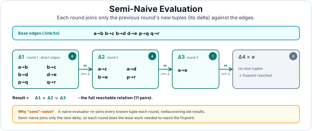
A naive bottom-up evaluator would keep rejoining all known reachable tuples in every round, rediscovering many results it already had. Semi-naive evaluation uses only the previous round's delta to produce the next delta, then unions the deltas into the final IDB relation. Chapter 9 shows the same idea with a longer reports-to example.
2.2 Magic-Set Rewrite
Now suppose the query asks only for nodes reachable from one bound start node, represented as a in the graph trace:
(def reachable-from-query
  '[:find [?end ...]
    :in $ % ?start
    :where (reachable ?start ?end)])

(d/q reachable-from-query db reachability-rules start-id)
import java.util.List;

Object reachableFromQuery = Datalevin.edn("""
    [:find [?end ...]
     :in $ % ?start
     :where (reachable ?start ?end)]
    """);

Object ends = conn.queryForm(reachableFromQuery,
    List.of(reachabilityRules, startId));
reachable_from_query = q.query(
    find=q.collection(end),
    inputs=[q.DB, q.RULES, start],
    where=[q.rule("reachable", start, end)],
)
ends = conn.query(reachable_from_query, reachability_rules, start_id)
const reachableFromQuery = q.query({
  find: q.collection(end),
  inputs: [q.DB, q.RULES, start],
  where: [q.rule("reachable", start, end)]
});
const ends = await conn.query(reachableFromQuery, reachabilityRules, startId);
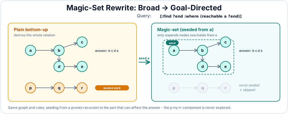
Plain bottom-up evaluation of reachable would also derive the disconnected p -> q -> r portion of the graph, even though it cannot affect the answer. A magic-set rewrite adds a temporary predicate that carries the bound arguments from the query into recursive evaluation. In this example, magic-reachable means "this start node can still contribute to the answer for the original query." Conceptually, the engine seeds that relation with the bound start node and threads it through the recursive rule:
;; Seed the temporary relation from the query binding:
;; only a is initially relevant.
(magic-reachable a)

;; If a relevant start has an outgoing edge, its neighbor can
;; become the start of a relevant recursive subcall.
[(magic-reachable ?mid)
 (magic-reachable ?start)
 [?start :link/to ?mid]]

;; Guard the original base rule so it only derives rows for relevant starts.
[(reachable ?start ?end)
 (magic-reachable ?start)
 [?start :link/to ?end]]

;; Guard the original recursive rule the same way.
[(reachable ?start ?end)
 (magic-reachable ?start)
 [?start :link/to ?mid]
 (reachable ?mid ?end)]
This is a conceptual rewrite, not Datalevin's literal internal representation, and magic-reachable is not a stored attribute, datom, or user-visible rule. It is an internal, temporary relation that marks which ?start values are worth expanding. Starting from a, the propagation rule discovers b, c, d, and e as relevant starts. The disconnected p, q, and r component is never marked, so the guarded reachable rules never derive rows for that component. The answers for the original query are still b, c, d, and e; the rewrite only avoids recursive work that cannot feed those answers.
Datalevin applies magic-set rewriting when a recursive rule call has bound arguments that can actually restrict recursive branches. If those bindings would not filter the recursive work, or if the magic relations grow beyond the optimizer's guardrail, the engine falls back to ordinary dependency-ordered recursive evaluation.
Figure 21.4 visually compares plain bottom-up evaluation with magic-set rewriting.
2.3 Rule Evaluation Refinements
Datalevin also connects rule evaluation back to the cost-based optimizer:
- Seeding tuples: Rule evaluation can receive bindings from earlier indexed query clauses. These seeds prevent unnecessary tuple generation and give recursion a warm start.
- Inlining non-recursive clauses: Clauses not involved in recursion can be pulled back into the ordinary query plan, where the cost-based optimizer can use indexes and join estimates.
- Early set boundaries and fused distinct operators: Each retained rule branch is projected to its head variables and deduplicated before branch results are combined. Where the shape permits, Datalevin fuses the join, projection, and distinct sink so duplicate proof paths are discarded as rows are produced instead of becoming a larger intermediate relation [12].
- Shape-specific EAV recursion: Eligible linear EAV branches can stream new candidates into their seen sets and reuse cached adjacency. Canonical transitive closure with one singleton-bound endpoint can traverse through EA or AV index probes and adapt to an attribute scan when observed fanout makes that cheaper. Synchronized two-link closures—recursive shapes that follow two EAV links in lockstep—have guarded demand-driven and dense bitset paths; other shapes retain general semi-naive evaluation [12].
- Proof-driven stopping and result collection: On a committed database, an eligible forward traversal can stop when its emitted answers saturate the exact AVE output domain. When a terminal result is also projected to the query's find variables and proven unique, Datalevin fully materializes it without repeating duplicate detection. Paths without those proofs keep the general evaluator and spillable set collector [12].
- Temporal elimination: Recursive rules that meet T-stratification criteria can keep only the last iteration's results, reducing memory use for long chains [10].
- Conservative complex clauses:
not,not-join,or, and function clauses obey the same binding discipline as ordinary queries. Recursive rules with negative or complex clauses use conservative planning paths rather than the positive-recursion magic-set path.
The practical takeaway is that rules are not interpreted as repeated application callbacks. They are compiled into set-oriented recursive evaluation, constrained by outer query bindings, and integrated with the same storage and planning principles used by ordinary Datalog queries.
3. Inspecting Query Plans with explain
Datalevin's query optimizer has good evidence, but it is still making estimates. Sometimes a query that should be fast takes longer than expected. To debug those cases, inspect the execution plan instead of guessing from the query text.
Datalevin's public diagnostic API for Datalog queries is explain. By default, explain plans the query without running it. When called with {:run? true}, it executes the same optimizer-selected physical alternative that an ordinary query would use and adds runtime measurements to the explain output.
| Entry point | Runs the query? | Physical-plan behavior |
|---|---|---|
Ordinary d/q |
Yes | Executes the selected conventional or access-path root and returns the query result. |
Plan-only d/explain |
No | Costs and selects a root, but does not execute it; :executed-plan-alternative has :kind :not-run. |
Measured d/explain with {:run? true} |
Yes | Executes the selected root, returns the result in the explain map, and reports the executed root and any runtime fallback. |
3.1 Plan-Only Explain
Use plan-only explain when you want to inspect join order, access paths, and estimated cardinalities without running the query itself.
(def query
  '[:find ?name
    :where [?e :user/name ?name]
           [?e :user/age ?age]
           [(> ?age 30)]])

(d/explain {} query (d/db conn))
String query =
    "[:find ?name " +
    " :where [?e :user/name ?name] " +
    "        [?e :user/age ?age] " +
    "        [(> ?age 30)]]";

Object plan = conn.explain(query);
from datalevin import q

(entity, name, age) = map(q.var, ("e", "name", "age"))
query = q.query(
    find=q.relation(name),
    where=[
        q.datom(entity, "user/name", name),
        q.datom(entity, "user/age", age),
        q.predicate(">", age, 30),
    ],
)

plan = conn.explain(query)
import { q } from "datalevin-node";

const entity = q.var("e");
const name = q.var("name");
const age = q.var("age");
const query = q.query({
  find: q.relation(name),
  where: [
    q.datom(entity, "user/name", name),
    q.datom(entity, "user/age", age),
    q.predicate(">", age, 30)
  ]
});

const plan = await conn.explain(query);
Plan-only output includes:
:query-graph: The optimizer's graph of clauses and estimated counts:plan: The fully planned conventional clause-and-join root, including its steps, join methods, estimated:cost, and estimated:size. It is also the ready fallback when an access root wins. The order of the:stepsis the chosen join order, and each step describes its join or index operation.- Access-path alternatives: When an AVE, idoc, full-text, or vector access expression is applicable,
:access-plansand:preferred-access-plandescribe its method, strategy, ordering, capabilities, candidate budget, and estimate.:physical-plan-alternativesshows the conventional and access roots compared by the cost model;:selected-plan-alternativeand:access-path-selected?identify the winner. - Selection versus execution:
:selected-plan-alternativeand:recommended-plan-alternativereport the optimizer's choice.:executed-plan-alternativehas:kind :not-runfor plan-only explain. :opt-clauses/:late-clauses: Clauses handled by the optimizer versus clauses processed after the optimized plan- Pre-planning rewrite decisions: When a constant AVE lookup is considered for early materialization,
:pre-materialization-decisionscompares its fan-out and complete candidate cost with leaving the lookup in the graph. - Planning times:
:parsing-time,:building-time,:planning-time, and:prepare-time
The actual value returned by explain is ordinary structured data and is much larger than what is useful to print inline. It includes the query graph, plan steps, rewritten clauses, timing fields, and many implementation details that are useful when debugging a specific query. The following is an abbreviated, human-friendly excerpt from the small query above:
{:planning-time "3.217",
 :opt-clauses
 [[?e :user/name ?name]
  [?e :user/age ?age]
  [(> ?age 30)]],
 :query-graph
 {$
  {?e
   {:free
    [{:attr :user/name, :var ?name}
     {:attr :user/age,
      :var ?age,
      :range [[[:open 30] [:closed :db.value/sysMax]]]}]}}},
 :plan
 {$
  [[{:steps
     ["Initialize [?e ?age] by range ... on :user/age."
      "Merge [?name] by scanning [:user/name]."],
     :cost nil,
     :size nil}]]},
 :late-clauses ()}
Read this in three parts. :late-clauses is empty, so the optimizer handled all clauses in the main plan. The predicate [(> ?age 30)] has been converted into a range bound on :user/age; it is not a separate row-by-row filter. The plan starts from that bounded age scan and then merges :user/name for the same entity. The :cost and :size fields can be nil for a single star-shaped component because there is no join-order competition to cost. In multi-component joins, :cost and :size are usually the main plan fields to inspect; in every case, the :query-graph count fields show the optimizer's estimated clause cardinalities.
Use plan-only explain to verify that a query is using the expected indexes and join strategies before running it on large data.
Use plan-only explain for large data
Plan-only diagnostics show the optimizer's intended access paths without executing the query. Use measured execution mode only when you are ready for the query to actually run.
3.2 Explain with Execution Measurements
Use {:run? true} when you also need measured execution information. This runs the query and augments the explain map with fields such as :execution-time, :actual-result-size, :result, and per-plan :actual-size where available.
(d/explain {:run? true} query (d/db conn))
import java.util.List;

Object measuredPlan = conn.explain("{:run? true}", query, List.of());
measured_plan = conn.explain(query, opts_edn="{:run? true}")
const measuredPlan = await conn.explain(query, {
  optsEdn: '{:run? true}'
});
{:run? true} is the runtime diagnostics mode of explain. It does not produce a separate clause-by-clause trace, but it lets you compare estimated sizes against actual sizes and distinguish planning cost from runtime cost.
For an ordered, limited AVE query like the one in Section 1.4, an abbreviated measured result can look like this. Unrelated fields are omitted:
{:selected-plan-alternative
 {:kind :access,
  :mode :adaptive-top-k,
  :size 7},
 :executed-plan-alternative
 {:kind :access,
  :mode :adaptive-top-k,
  :size 7},
 :plan
 {:kind :access,
  :mode :adaptive-top-k,
  :access-plan {:method :ave},
  :size 7,
  :actual-size 6,
  :candidate-count 360,
  :fragment-result-count 215,
  :residual-result-count 215},
 :actual-result-size 6}
The selected summary records the optimizer's choice; the executed summary confirms which root actually ran. Inside :plan, :size 7 is the estimated output of that access root and :actual-size 6 is its measured output. The source admitted 360 candidate tuples, the access fragment produced 215, and the residual query also produced 215. Applying final ordering and :limit returned six rows. Candidate, fragment, and residual counts describe successive stages of one pipeline; they are not alternative estimates of the same relation.
If the conventional root wins, :plan retains the grouped component plans and measured execution adds :actual-size where available. If an access root wins, :plan has :kind :access and identifies its :mode and :access-plan. Additional fields such as :candidate-work, :batches, and :subqueries provide progressively more detail when needed.
An adaptive access execution can still exhaust its candidate budget or safety cap and continue with the already planned conventional root. In that case, :plan preserves the attempted access work and adds :fallback; the same fallback is attached to :executed-plan-alternative, and the conventional fallback plan appears among :subqueries. Thus the measured plan describes the path actually taken rather than attributing conventional counts to the selected access root.
When eligible late indexed producers compete with a bound pattern, :late-clause-decisions records whether Datalevin kept the bound pattern first or selected an indexed union or range first, along with the runtime cost inputs. The decision can depend on values and relation sizes available only at that boundary. Morsel-specific :partitioned-execution fields are documented with morsel-driven execution in Section 1.7.1.
Compare estimated and actual fields at the same nesting level. Use :actual-result-size for the final measured cardinality and :prepare-time versus :execution-time to separate planning overhead from execution time. When corresponding estimated and actual sizes are close, the planner's model matched the current data. Datalevin is normally very accurate in the first few plan steps because it can combine exact index counts with query-specific sampling, and those early steps matter most for keeping intermediate results small.
If :size and :actual-size differ by orders of magnitude, cardinality estimation was wrong for that part of the plan. The cause may be a predicate or a join whose selectivity is hard to estimate, but it can also be stale or sparse attribute metadata: Datalevin refreshes per-attribute eid samples, attribute cardinality counters, and default fan-out ratios in the background, and a very fast load or major reshaping of data may outrun that process. Background sampling is enabled by default, but explicit analyze is useful when you need those statistics refreshed before judging a plan. After a bulk load or major reshaping of data, refresh statistics for the affected attribute, or for the database as a whole:
(d/analyze (d/db conn) :user/age)
(d/analyze (d/db conn))
conn.analyze(":user/age");
conn.analyze();
conn.analyze(":user/age")
conn.analyze()
await conn.analyze(':user/age');
await conn.analyze();
3.3 Understanding Join Orders
The :plan section shows the join order chosen by the optimizer.
- Leading Clause: This is the first clause the engine used to find the initial set of entities.
- Sequential Joins: The order in which subsequent clauses were applied.
If you see that the engine is starting with a non-selective clause (e.g., searching for :user/active? true), it might be because the selective filter you expect is hidden inside a complex predicate or rule.
A common join-order bottleneck is a large intermediate result set. If the first join returns 1,000,000 entities, but the second join filters them down to 10, the engine still had to process 1,000,000 records.
The fix is to ask whether the query can express a more selective indexed constraint earlier in the plan. The optimizer tries to do this automatically, but a complex predicate or rule may hide the selective condition from estimation.
3.4 Diagnosing Slow Predicates
Some custom predicates are visible to the optimizer. A predicate that can be pushed down, typically one involving a single free variable and no source expression, is executed during query-specific sampling, so Datalevin can estimate its selectivity from the current data. For example, a predicate such as [(my-ns/is-complex? ?x)] can be planned differently from a late filter when ?x is attached to a sampled value path.
The harder cases are predicates that cannot be pushed down, such as predicates over several variables, predicates that depend on an explicit source, or functions whose own runtime cost dominates even when selectivity is estimated well. explain can show whether the predicate became part of the optimized plan or remained in :late-clauses, but it does not time each predicate call separately. If a query becomes slow only after adding a predicate, isolate that predicate by comparing explain output and query runtime before and after adding it.
Filter before expensive predicates
Prefer indexed constraints that reduce the candidate set before expensive
non-pushdownable predicates run. If a predicate makes a query slow, compare
explain output and runtime before and after adding that predicate.
3.5 Repeated Reads with Prepared Queries
If a request handler repeatedly runs the same query with different inputs, prepare it once with d/prepare-q. Call d/execute-prepared for each request, passing the remaining inputs in a vector. Compare response times using typical inputs to see whether preparation helps your workload. Queries that read or return large amounts of data still benefit from more selective conditions and smaller result sets.
Chapter 7, Section 5 covers these Datalevin 1.2.0 APIs, along with prepare-pull, prepare-get-value, input conventions, and remote execution.
4. Related Benchmark Coverage
For performance evidence, see Chapter 1 for the Join Order Benchmark, Chapter 9 for OpenRuleBench, and Chapter 13 for LDBC SNB. This chapter stays focused on planner mechanics and the explain workflow.
Summary
The chapter has three layers: optimizer mechanics, recursive-rule evaluation, and the practical diagnostics workflow. When a query is slow, follow this workflow:
- Use plan-only
explain: Inspect join methods, index usage, and estimated cardinalities. For bounded queries, also inspect:access-path-selected?, the preferred method and strategy, and the selected adaptive mode. When present, inspect:pre-materialization-decisionsfor selective AVE anchors. - Use
explainwith{:run? true}: Confirm the executed root in:executed-plan-alternative, then compare estimates with actual result sizes and total execution time. For an access root, inspect its method, mode, candidate counts, batches, residual subqueries, and any fallback. Check:late-clause-decisionswhen the query has a late indexed union or bounded range. For a large read-only component plan,:partitioned-executionconfirms whether an eligible linear segment was divided into morsels. - Check cardinality gaps: Large gaps between estimated
:sizeand measured:actual-sizeare a strong hint that a predicate, rule, stale per-attribute sample, or rapidly changed data is hiding selectivity from the optimizer. If the data changed quickly, rund/analyzebefore drawing conclusions from the plan. - Simplify and isolate: Remove clauses one by one to find the specific part of the query that is slow.
- Refine the logic: Prefer more selective indexed attributes to expensive custom predicates.
By using explain well, you gain the transparency needed to understand how Datalevin plans a query and why a query may be slower than expected.
References
[1] Patricia G. Selinger, Morton M. Astrahan, Donald D. Chamberlin, Raymond A. Lorie, and Thomas G. Price, "Access Path Selection in a Relational Database Management System," SIGMOD 1979, pp. 23-34. URL: https://research.ibm.com/publications/access-path-selection-in-a-relational-database-management-system. DOI: https://doi.org/10.1145/582095.582099.
[2] Guido Moerkotte and Thomas Neumann, "Dynamic Programming Strikes Back," SIGMOD 2008, pp. 539-552.
[3] Hai Lan, Zhifeng Bao, and Yuwei Peng, "A Survey on Advancing the DBMS Query Optimizer: Cardinality Estimation, Cost Model, and Plan Enumeration," Data Science and Engineering, 2021.
[4] Andreas Brodt, Oliver Schiller, and Bernhard Mitschang, "Efficient Resource Attribute Retrieval in RDF Triple Stores," CIKM 2011, pp. 1445-1454.
[5] Andrey Gubichev and Thomas Neumann, "Exploiting the Query Structure for Efficient Join Ordering in SPARQL Queries," EDBT 2014.
[6] Marios Meimaris et al., "Extended Characteristic Sets: Graph Indexing for SPARQL Query Optimization," ICDE 2017.
[7] Thomas Neumann and Guido Moerkotte, "Characteristic Sets: Accurate Cardinality Estimation for RDF Queries with Multiple Joins," ICDE 2011.
[8] Todd J. Green, Shan Shan Huang, Boon Thau Loo, and Wenchao Zhou, "Datalog and Recursive Query Processing," Foundations and Trends in Databases 5(2):105-195, 2013. URL: https://www.nowpublishers.com/article/Details/DBS-017. DOI: https://doi.org/10.1561/1900000017.
[9] Francois Bancilhon, David Maier, Yehoshua Sagiv, and Jeffrey D. Ullman, "Magic Sets and Other Strange Ways to Implement Logic Programs," PODS 1986, pp. 1-15. DOI: https://doi.org/10.1145/6012.15399.
[10] Amir Shaikhha et al., "Optimizing Nested Recursive Queries," Proceedings of the ACM on Management of Data 2(1), SIGMOD 2024, pp. 1-27.
[11] Datalevin project, "Query Processing," parallel-processing design and execution diagnostics, commit ee208cec. URL: https://github.com/datalevin/datalevin/blob/ee208cecb3378da5c843e4ebbcb9bcd372516ef4/doc/query.md#parallel-processing.
[12] Datalevin project, "Datalevin Rule Engine," implementation notes. URL: https://github.com/datalevin/datalevin/blob/master/doc/rules.md.
User Examples
Log in to create examplesNo examples for this chapter yet.